Prof. Upinder S. Bhalla - Kinetikit Examples
Here are some simulations from the 'examples' directory for the kinetics package.
Contents
- Bistable feedback model.
- Bistable inhibitory feedback loop model.
- Example of transporter object.
- Example of end-product inhibition.
- Example of large research simulation.
feedback.g : Feedback model with bistability. Described in the tutorial document and in the corresponding chapter for the Book of Genesis.
Bistable feedback loop reaction diagram.
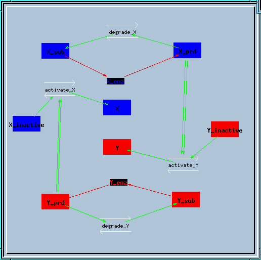
This is the structure of the feedback loop. The enzyme X creates a produce X_prd, which activates enzyme Y in a second-order manner. Similarly, enzyme Y produces Y_prd to activate X.
Output of the feedback loop.
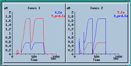
This is a plot of the output of the feedback loop. In this simulation, a small input was initially applied at t = 100. The input was applied by setting the concentration of X_prd to 1. This is equivalent to an instantaneous application of this amount of X_prd, without any buffering. This stimulus failed to activate the feedback loop. Then a large input (X_prd = 2) was applied at t=200. The feedback loop turned on. At t = 400, a small inhibitory input was applied (buffer X_prd to zero for 10 sec). The activity of the feedback loop recovered after this stimulus, and went back to the upper activity state. Finally, at t= 700, a large inhibitory input was applied by buffering X_prd to zero for 50 sec. The loop turned off again.
inhib_fb.g : Inhibitory feedback model, which also exhibits bistability.
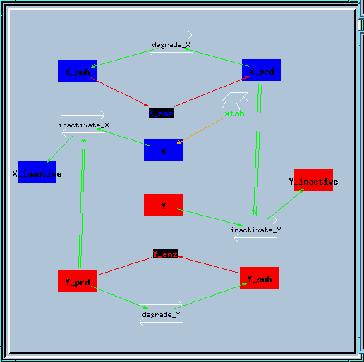
It has only a couple of minor changes with respect to the feedback.g model. This model also contains a table set up to give step inputs for generating a conc-eff curve. This table is not activated by default; you will need to double-click the table icon and turn the stimulus ON to get it to work.
Bistable inhibitory feedback loop reaction diagram.
Running the model with a concentration step series.
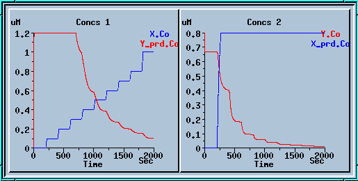
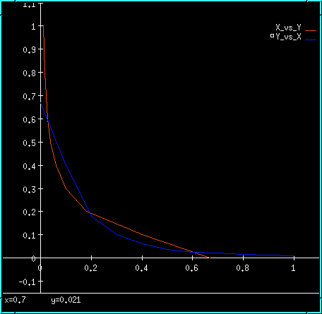
These plots display the output of the model with the table ON. The blue plot on the left is the value of enzyme X, which is controlled by the table. The red plot on the right is the output concentration of enzyme Y. If you were to take the steady-state Y concentrations for each value of X and plot them, you would get an intersecting curve like the one below:
Inhibitory feedback bistability plot.
The model has the very neat property that it will happily go into the metastable state when it is started up without any changes. If one now alters the last digit of the conc term on X or Y (or if you want to be really clean, on X_prd or Y_prd), the symmetry is broken and the system falls into one of the true bistable states. Try it out:
Symmetry breaking with a small increase to x_prd.
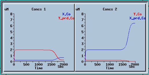
Here we ran the model for 1000 sec, applied a small increase to x_prd, and ran for another 1000 sec.
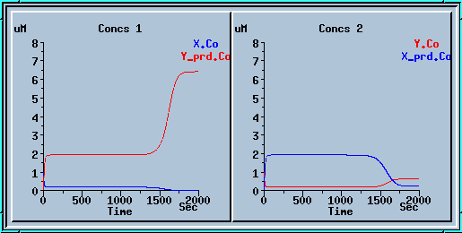
In the example below we ran the model for 1000 sec, applied a small decrease to x_prd, and ran for another 1000 sec. We get a nice mirror image of the previous run.
Symmetry breaking with a small decrease to x_prd.
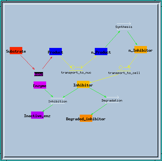
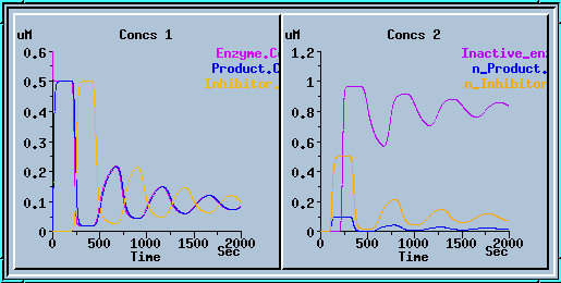
transport.g : Example of using the transporter element. Requires at least GENESIS 2.2. This simulates the translocation of an enzyme product to the nucleus, which results in synthesis of a blocker, which is transported back to the cytoplasm to block the enzyme. You get a nice series of decaying oscillations.
Transporter model.
Transporter simulation.
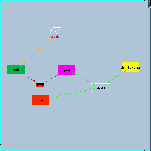
end_prd_inhib.g : Example of end-product inhibition from the tutorial in sections 2, 3 and 4.
End-product inhibition model.
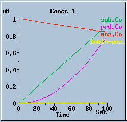
End-product inhibition: Comparison of response with and without inhibition.
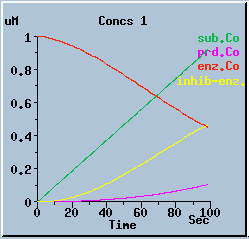
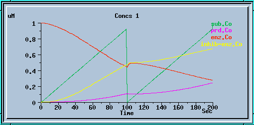
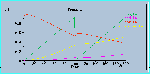
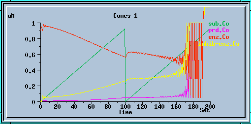
The following graphs are the response with inhibition activated, at different timesteps. These plots illustrate the loss of accuracy and stability as timesteps become larger. All these runs were carried out using the default exponential Euler integration method.
End-product inhibition: Accurate response at dt = 0.01 sec.
End-product inhibition: Inaccurate response at dt = 0.5 sec.
End-product inhibition: Unstable response at dt = 1 sec.
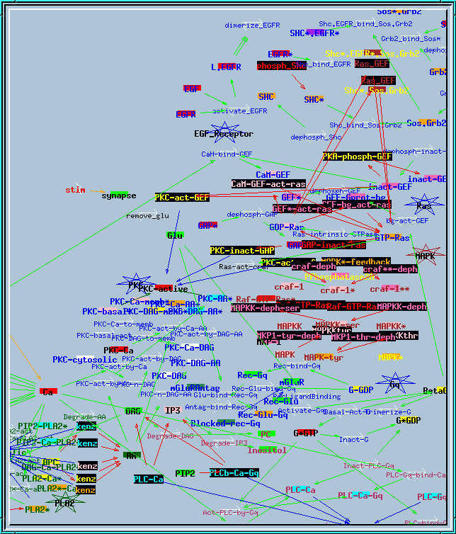
all117.g : Example of large research simulation from Bhalla and Iyengar, Science 1999. It needs variable timesteps with small initial dt to run properly. This screen shot of the reaction network actually shows only about half of the reactions and pools.
Synaptic signaling model.
